We talked about the basics of SVM in the
previous blog, and now let's use an example to show you how to use it easily with
sklearn, and also, some of the important parameters of it. You can find all the code at
Qingkai's Github.
import numpy as np
import itertools
import matplotlib.pyplot as plt
from sklearn import svm, datasets
from sklearn.cross_validation import train_test_split
from sklearn.preprocessing import StandardScaler
from sklearn.metrics import classification_report,confusion_matrix
plt.style.use('seaborn-poster')
%matplotlib inline
Load and visualize data
Let's load the
IRIS from sklearn. This dataset is a very famous dataset for pattern recognition that from the famous
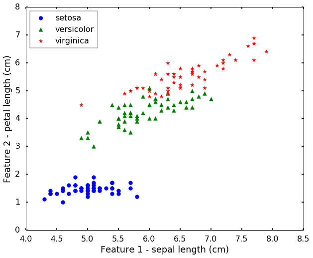
Fisher's paper in 1936. The data set contains 3 classes of 50 instances each, where each class refers to a type of iris plant. The features are Sepal Length, Sepal Width, Petal Length and Petal Width. They are related with the physical properties of the plant. Today we will use only 2 features for easy visualization purposes.
iris = datasets.load_iris()
X = iris.data[:, [0, 2]]
y = iris.target
target_names = iris.target_names
feature_names = iris.feature_names
n_class = len(set(y))
print('We have %d classes in the data'%(n_class))
We have 3 classes in the data
plt.figure(figsize = (10,8))
for i, c, s in (zip(range(n_class), ['b', 'g', 'r'], ['o', '^', '*'])):
ix = y == i
plt.scatter(X[:, 0][ix], X[:, 1][ix], color = c, marker = s, s = 60, label = target_names[i])
plt.legend(loc = 2, scatterpoints = 1)
plt.xlabel('Feature 1 - ' + feature_names[0])
plt.ylabel('Feature 2 - ' + feature_names[2])
plt.show()
Train an SVM classifier
Since our purpose is to understand the SVM classifier, therefore, we won't split the data into training, validation, and test dataset. Also, we will not scale the data, because the values are all similar. (In reality, you still want this in your workflow, and use cross-validation or gridsearch to determine some parameters). Here, let's just train the SVM classifier directly.
clf = svm.SVC(kernel='linear')
clf.fit(X,y)
SVC(C=1.0, cache_size=200, class_weight=None, coef0=0.0,
  decision_function_shape=None, degree=3, gamma='auto', kernel='linear',
  max_iter=-1, probability=False, random_state=None, shrinking=True,
  tol=0.001, verbose=False)
The training results
Let's view the performance on the training data, we will plot the
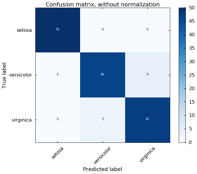
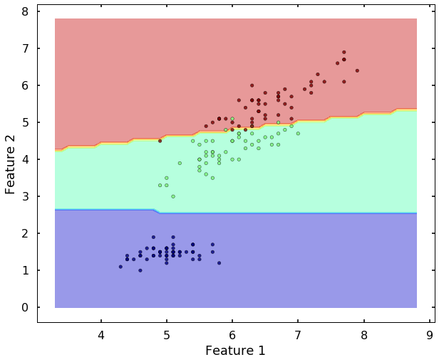
confusion matrix. Also, we will plot the decision boundary, which will help us understand more of the capability of the classifier (since we only have two selected features, this makes us easier to view the decision boundary).
def plot_confusion_matrix(cm, classes,
normalize=False,
title='Confusion matrix',
cmap=plt.cm.Blues):
"""
This function prints and plots the confusion matrix.
Normalization can be applied by setting `normalize=True`.
"""
fig = plt.figure(figsize=(10, 8))
plt.imshow(cm, interpolation='nearest', cmap=cmap)
plt.title(title)
plt.colorbar()
tick_marks = np.arange(len(classes))
plt.xticks(tick_marks, classes, rotation=45)
plt.yticks(tick_marks, classes)
if normalize:
cm = cm.astype('float') / cm.sum(axis=1)[:, np.newaxis]
thresh = cm.max() / 2.
for i, j in itertools.product(range(cm.shape[0]), range(cm.shape[1])):
plt.text(j, i, cm[i, j],
horizontalalignment="center",
color="white" if cm[i, j] > thresh else "black")
plt.tight_layout()
plt.ylabel('True label')
plt.xlabel('Predicted label')
plt.show()
def plot_desicion_boundary(X, y, clf, title = None):
'''
Helper function to plot the decision boundary for the SVM
'''
x_min, x_max = X[:, 0].min() - 1, X[:, 0].max() + 1
y_min, y_max = X[:, 1].min() - 1, X[:, 1].max() + 1
xx, yy = np.meshgrid(np.arange(x_min, x_max, 0.1),
np.arange(y_min, y_max, 0.1))
Z = clf.predict(np.c_[xx.ravel(), yy.ravel()])
Z = Z.reshape(xx.shape)
plt.figure(figsize = (10, 8))
plt.contourf(xx, yy, Z, alpha=0.4)
plt.scatter(X[:, 0], X[:, 1], c=y, alpha=0.8)
if title is not None:
plt.title(title)
plt.xlabel('Feature 1')
plt.ylabel('Feature 2')
plt.show()
predicted = clf.predict(X)
cm = confusion_matrix(y,predicted)
plot_confusion_matrix(cm, classes=iris.target_names,
title='Confusion matrix, without normalization')
plot_desicion_boundary(X, y, clf)
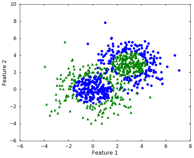
We can see the above two figures, the SVM classifier actually did a decent job to separate different classes. Since the data is linearly separatable, the 'linear' kernel can satisfy the job. But what if the data is not linearly separatable? Let's see another example.
Non-linearly separatable example
X1, y1 = datasets.make_gaussian_quantiles(cov=2.,
n_samples=400, n_features=2,
n_classes=2, random_state=1)
X2, y2 = datasets.make_gaussian_quantiles(mean=(3, 3), cov=1.5,
n_samples=400, n_features=2,
n_classes=2, random_state=1)
X = np.concatenate((X1, X2))
y = np.concatenate((y1, - y2 + 1))
n_class = 2
plt.figure(figsize = (10,8))
for i, c, s in (zip(range(n_class), ['b', 'g'], ['o', '^'])):
ix = y == i
plt.scatter(X[:, 0][ix], X[:, 1][ix], color = c, marker = s, s = 60)
plt.xlabel('Feature 1')
plt.ylabel('Feature 2')
plt.show()
clf = svm.SVC(kernel='linear')
clf.fit(X,y)
SVC(C=1.0, cache_size=200, class_weight=None, coef0=0.0,
  decision_function_shape=None, degree=3, gamma='auto', kernel='linear',
  max_iter=-1, probability=False, random_state=None, shrinking=True,
  tol=0.001, verbose=False)
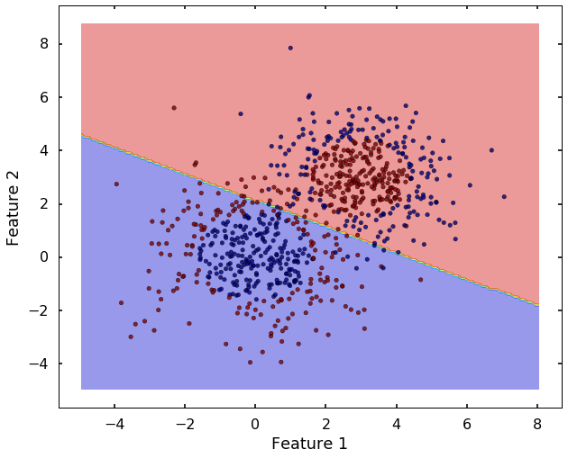
plot_desicion_boundary(X, y, clf)
Now we can see that, the 'linear' kernel is not working anymore. It tries to use a linear boundary to classify the data, which is impossible. Remembered that we talked in the previous blog that using a different kernel will transform this data into higher dimensions to separate them linearly. There are a couple of options in sklearn to choose, the most popular ones are
'rbf' - radial basis function,
'poly' - the polynomial. We will use 'rbf' here.
clf = svm.SVC(kernel='rbf')
clf.fit(X,y)
SVC(C=1.0, cache_size=200, class_weight=None, coef0=0.0,
  decision_function_shape=None, degree=3, gamma='auto', kernel='rbf',
  max_iter=-1, probability=False, random_state=None, shrinking=True,
  tol=0.001, verbose=False)
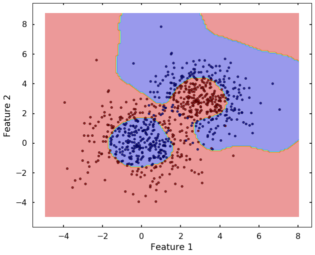
plot_desicion_boundary(X, y, clf)
Haha, after we used the 'rbf' kernel, it seems the SVM can classify them much better. The 'rbf' kernel based SVM looks much flexible, but it also more prone to
overfit the data. Therefore, to better use it, you need understand two important parameters: C and gamma, let's have a closer look at them.
C and gamma in SVM
The C and gamma parameter in the SVM are the most important parameters for the 'rbf' kernel, that can be determined by the grid-search method. But we need get a sense how they affect the results if we change them.
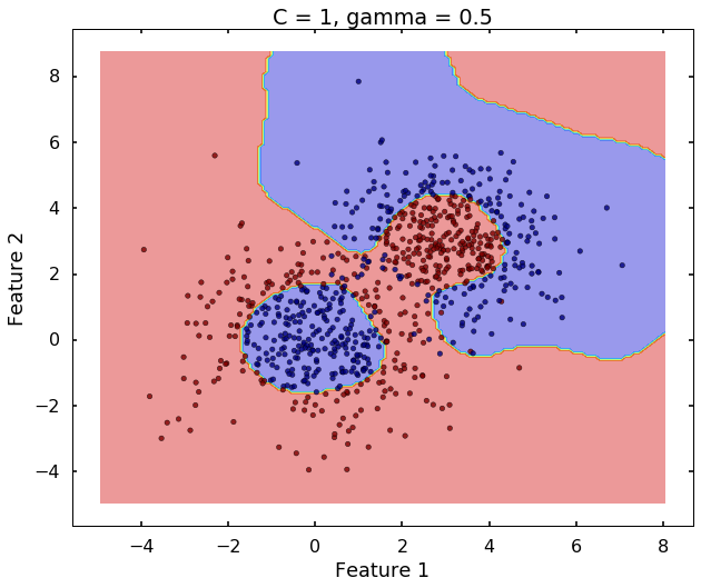
C controls the cost of misclassification on the training data, it trades off misclassification on training examples against simplicity of the decision boundary. A large C makes the cost of misclassification high, this will force the algorithm to fit the data with more flexible model, and try to classify the training data correctly as much as possible. But this will also make the SVM more easier to overit the data. Therefore, the simple rule to remember is:
- Larger C, lower bias, higher variance.
- Smaller C, higher bias, lower variance.
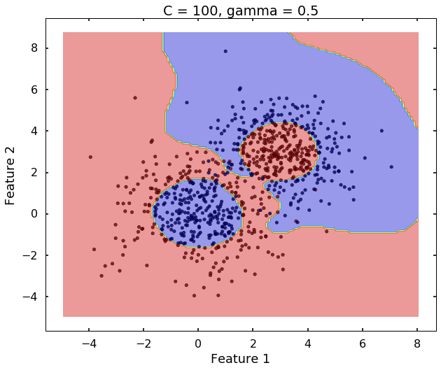
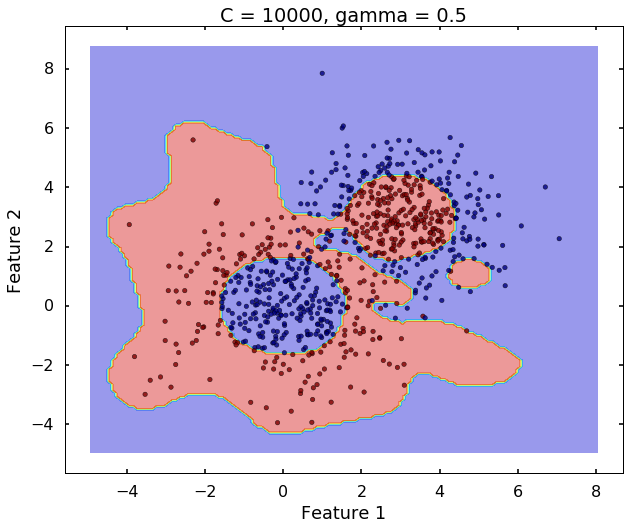
The following 3 figures showing different values of C, that is, C = 1, C = 100, C = 10000. We can see the higher the value C, the more complicated the decision boundary is, which tries to fit every training data, even with some clearly anomaly data.
clf = svm.SVC(kernel='rbf', C = 1, gamma = 0.5)
clf.fit(X,y)
plot_desicion_boundary(X, y, clf, title = 'C = 1, gamma = 0.5')
clf = svm.SVC(kernel='rbf', C = 100, gamma = 0.5)
clf.fit(X,y)
plot_desicion_boundary(X, y, clf, title = 'C = 100, gamma = 0.5')
clf = svm.SVC(kernel='rbf', C = 10000, gamma = 0.5)
clf.fit(X,y)
plot_desicion_boundary(X, y, clf, title = 'C = 10000, gamma = 0.5')


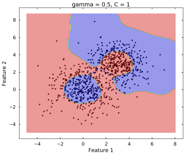
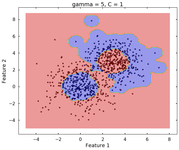
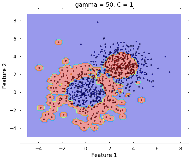
Technically, gamma is not a parameter of the SVM, but a parameter for the 'rbf' kernel to handle non-linear classification. It defines how far the influence of a single training example reaches. A low value of gamma means 'far' and high value means 'close'. Therefore, A small gamma means a radial basis function with far influence, i.e. if x is a support vector, a small gamma implies the class of this support vector will have influence on deciding the class of the vector y even if the distance between them is large. If gamma is large, then variance is small implying the support vector does not have wide-spread influence. A rule to remember:
- large gamma leads to high bias and low variance
- small gamma leads to low bias and high variance
clf = svm.SVC(kernel='rbf', gamma = 0.5, C = 1)
clf.fit(X,y)
plot_desicion_boundary(X, y, clf, title = 'gamma = 0.5, C = 1')
clf = svm.SVC(kernel='rbf', gamma = 5, C = 1)
clf.fit(X,y)
plot_desicion_boundary(X, y, clf, title = 'gamma = 5, C = 1')
clf = svm.SVC(kernel='rbf', gamma = 50, C = 1)
clf.fit(X,y)
plot_desicion_boundary(X, y, clf, title = 'gamma = 50, C = 1')
More on the parameters
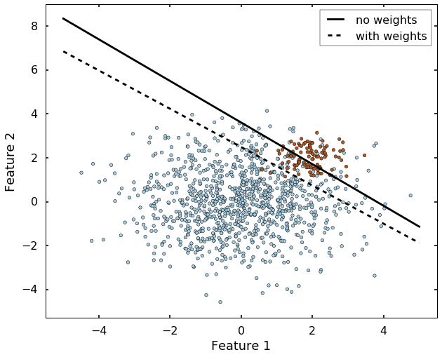
Another very important parameter is the class_weight, which will address the inbalance class case. Let's see an extreme example: if we have 99 instances of class 0, but 1 instance of class 1, then even the algorithm classify everything to class 0, we will have 99% correct rate. This is always the case if we have an inbalanced dataset, there are many ways to deal with it, but the parameter 'class_weight' in SVM will deal with this case by setting different weights to different classes. Let's grab the example from
sklearn website directly. We can see without specify the class_weight, the boundary is set where most of the blue dots on beneath the boundary. But after we specified the class_weight, the SVM now pays more attention to the minor class (class 1), and classify most of them correct.
rng = np.random.RandomState(0)
n_samples_1 = 1000
n_samples_2 = 100
X = np.r_[1.5 * rng.randn(n_samples_1, 2),
0.5 * rng.randn(n_samples_2, 2) + [2, 2]]
y = [0] * (n_samples_1) + [1] * (n_samples_2)
clf = svm.SVC(kernel='linear', C=1.0)
clf.fit(X, y)
w = clf.coef_[0]
a = -w[0] / w[1]
xx = np.linspace(-5, 5)
yy = a * xx - clf.intercept_[0] / w[1]
wclf = svm.SVC(kernel='linear', class_weight={1: 10})
wclf.fit(X, y)
ww = wclf.coef_[0]
wa = -ww[0] / ww[1]
wyy = wa * xx - wclf.intercept_[0] / ww[1]
plt.figure(figsize = (10, 8))
h0 = plt.plot(xx, yy, 'k-', label='no weights')
h1 = plt.plot(xx, wyy, 'k--', label='with weights')
plt.scatter(X[:, 0], X[:, 1], c=y, cmap=plt.cm.Paired)
plt.legend()
plt.xlabel('Feature 1')
plt.ylabel('Feature 2')
plt.axis('tight')
plt.show()
References
