Mining Gmail using Python (only timestamp)

Today I had a presentation at The Hacker Within Berkeley about a simple mining of your Gmail emails arriving/sending time using python. You can download the notebook at Qingkai's Github. The idea is to find some patterns from the emails I received/sent. I only use the timestamp associated with the emails, but you can use other information as well. The data I used is the entire inbox and sent box, which happens to be my PhD life, since I registered my Gmail when I started my PhD here.

1 Distribution of the emails through out the day
The following two figures shows the distribution of my incoming/outgoing emails during the day, I have 3 peaks, one in the late morning, one in the afternoon, and one before sleep.

2 Distribution of the emails through out the period
The following two figures shows when the emails comes in from 2012 - 2016, some imedieate features are:
(1) we see gaps for the summer/winter breaks
(2) some emails come in at fixed time from automatic services
(3) I do seem have more emails with time progress

3 Aggregate the count 
The following two figures shows the number of emails aggregated by day and by month. You can see the high frequency changes on the daily plot, and the low frequency on the monthly plot. It seems the outgoing emails correlate the incoming emails very well. And indeed, there's a trend that I received more and more emails.

4 Regression
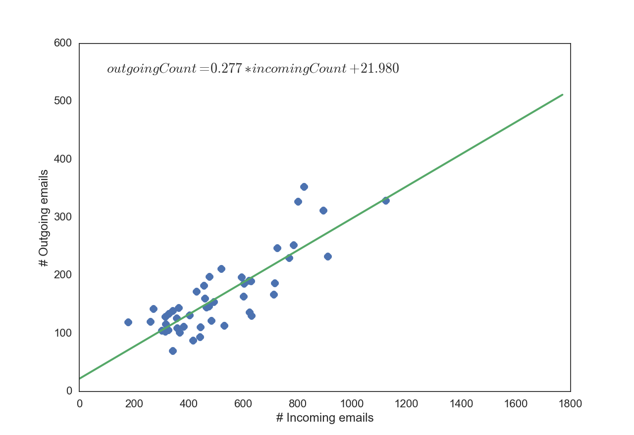
The following figure shows the relationship between the incoming and outgoing emails. It seems that for every 100 emails I received, and I will sent about 28 emails.

5 Finding the repeating pattern
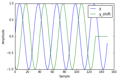
The following figure shows the FFT spectrum of the emails I sent out. And I also labeled the top 5 peaks which corresponding to 1 week, half year, full year, 8 months, and half week.  Can you tell why they repeat?

6 Do I changed my sending email behavior?
Looking at the first figure, do you think I changed my behavior of sending emails? We can model this data and try to answer this question by using the Bayesian analysis (see the notebooks for details). The basic idea is to find a month that may mark as the switch point, that the months before it I sent emails differently from that after it. So using a poisson distribution to model the count data, and a uniform distribution to reflect we have no information for this switch point at all, we did a MCMC sampling of the posterior distribution of these parameters, which shows in the second figure, and we can see it point to the 20th month as my switch month. This happens to be the time when I finish my qualify exam, and started a new semester. Now you can see that PhD life is totally different before and after the qualify exam, and it even shown on my email data!!!

The Code That Runs Our Lives

Did you use deep learning today?

Signal Processing: Shift a signal in the frequency domain

Shift signal in frequency domain¶

We need shift an signal for many cases, i.e. when we calculate cross correlation between signals, when we do beamforming to find out the direction of the energy comes, when we use back-projection to track the source of an earthquake, etc. One easy way to shift the signal is in the frequency domain. In this blog, I will show you how to shift an signal in the frequency domain. You can find the script at Qingkai's Github.

The theory behind it¶

When we do a Fast Fourier Transform (FFT), we actually map a finite length of time domain samples into an equal length sequence of frequency domain samples.
$$X[k]=\sum_{n = 0}^{N−1} x[n]e^{\frac{−j2πnk}{N}}=A_ke^{jϕ_k}$$
A property of the Fourier transform is that, a delay in the time domain maps to a phase shift in the frequency domain. For the DFT, this property is:
$$x[n]↔X[k]$$$$x[n−D]↔e^{\frac{−j2πnkD}{N}}X[k]$$
This is to say, if we delay our input signal by D samples in the time domain, it is equavalent to each complex value in the FFT of the signal is multiplied by the constant $$e^{\frac{−j2πnkD}{N}}$$.

In [1]:

import matplotlib.pyplot as plt
import numpy as np

In [2]:

def nextpow2(i):
    '''
    Find the next power 2 number for FFT
    '''
    
    n = 1
    while n < i: n *= 2
    return n

def shift_signal_in_frequency_domain(datin, shift):
    '''
    This is function to shift a signal in frequency domain. 
    The idea is in the frequency domain, 
    we just multiply the signal with the phase shift. 
    '''
    Nin = len(datin) 
    
    # get the next power 2 number for fft
    N = nextpow2(Nin +np.max(np.abs(shift)))
    
    # do the fft
    fdatin = np.fft.fft(datin, N)
    
    # get the phase shift for the signal, shift here is D in the above explaination
    ik = np.array([2j*np.pi*k for k in xrange(0, N)]) / N 
    fshift = np.exp(-ik*shift)
        
    # multiple the signal with the shift and transform it back to time domain
    datout = np.real(np.fft.ifft(fshift * fdatin))
    
    # only get the data have the same length as the input signal
    datout = datout[0:Nin]
    
    return datout

Example¶

In [3]:

Fs = 150.0;  # sampling rate
Ts = 1.0/Fs; # sampling interval
t = np.arange(0,1,Ts) # time vector

ff = 5;   # frequency of the signal

# let's generate a sine signal
y = np.sin(2*np.pi*ff*t)

# shift the signal in the frequency domain by 20 samples
y_shift = shift_signal_in_frequency_domain(y, -20)

plt.plot(y, label = 'y')
plt.plot(y_shift, label = 'y_shift')
plt.xlabel('Sample')
plt.ylabel('Amplitude')
plt.legend()
plt.show()

References¶

Good explaination at stackexchange: http://dsp.stackexchange.com/questions/509/what-effect-does-a-delay-in-the-time-domain-have-in-the-frequency-domain