Tuesday, June 26, 2018

Difference of gasoline when you fill in at different temperatures

We know objects are expanding when the temperature goes up. Therefore, I always think that I should fill in my gasoline in my car in the early morning so that I could have more gasoline when I spend the same money. But how much really we could gain if the temperature changes fill in gasoline at 60°F instead of 80°F (this is actually the changes of temperature at Berkeley during the morning and noon). I want to have a rough estimation of what's the difference between the amount of gasoline when I fill in at different times of the day. To calculate the change of the gasoline, we need to use the physics that we learned in high school, the basic equation is the following one, that relates the volume change of an object to the temperature change.
\Delta = \beta\times T \times \DeltaT
\DeltaV is the change of the volume, and \beta is the average coefficient of volume expansion, and the V is the initial volume of the object, and \DeltaT is the change of the temperature. Therefore, all we need to do is to find the coefficient of volume expansion, and it is 9.6\times 10^{-4}/C°, that is 5.33\times 10^{-4}/F°. Now, let’s assume that we fill in 10-gallon gasoline in the morning at 60°F and how much it will be at noon (80°F)
delta_v = 5.33e-4 * 10 * (80-60)
print('We gain %.2f gallon gasoline, \nif we fill in the morning instead of noon.'%delta_v)
We gain 0.11 gallon gasoline, 
if we fill in the morning instead of noon.
Well, it is 0.11-gallon difference if we fill in 10-gallon gasoline in the morning (that is, we will have 10.11 gallon at noon when temperature increases to 80°F). Let’s calculate how much we potentially can save if we drive our car for certain distances.
Let’s say your car’s average MPG is 30, for 150,000 miles, we need 150,000 / 30 = 5000-gallon gasoline. The difference of gasoline will be 5000 / 10 \times0.11 = 55gallon.

Saturday, June 23, 2018

Quick guide of Python classes

This week, I will give some examples of the object-oriented programming part of Python. The object-oriented programming has many advantages. And I really like them due to the reusability of the code and the feeling of modeling the world :-). I will give some examples that I usually use in my code as a quick guide of how to use these in your code. This tutorial serves as a quick guide, if you want to learn more, you should go to the documentation. 

Define a class

Let's start to look at the following examples, where we create a People class. 
class People(object):
    
    def __init__(self, name, age):
        self.name = name
        self.age = age
        
    def greet(self):
        print("Greetings, " + self.name)
Typical python class has a constructor, that is the _init_() function, which initializes the class when you call it. This means that, when you first initialize your class, this function will be only run once. The 'self' means the instance itself, you can find a very good explanation here. The self.name and self.age are the attributes that the class will have, you can see from the following example. And the greet function is the method that we define in the class. Let's see how we can actually use it. 
person1 = People(name = 'Iron Man', age = 35)
person1.greet()
print(person1.name)
Greetings, Iron Man
Iron Man

Inheritance

One of the most important features of using the object-oriented programming is that we can easily reuse the code above to create some new classes. For example, we want to have another class Teacher that have all the attributes and methods People class have, but at the same time, we want to have more new methods. 
class Teacher(People):
    
    def teach_students(self, x, y):
        print('x + y = %d'%(x+y))
teacher1 = Teacher(name = 'Susan', age = 24)
teacher1.greet()
teacher1.teach_students(x = 3, y = 5)
Greetings, Susan
x + y = 8
We can see from the above code that, we don't need to re-define all the attributes and greet function, the Teacher class actually have all these from People class, this is due to this line: class Teacher(People), which basically say that we want Teacher class to get all the things from People class. This is called inherit, and class Teacher inherits from class People. And People is the parent class and Teacher is a child class. And then we could extend the methods in class Teacher by just define new functions. Or if we want to replace some of the old methods in People, all we need to do is to re-define the function, for example, in the following lines, we replace the greet method in People with a new one that greet the teacher. 
class Teacher(People):
    
    def greet(self):
        print("Greetings, teacher: " + self.name)
    
    def teach_students(self, x, y):
        print('x + y = %d'%(x+y))
teacher1 = Teacher(name = 'Susan', age = 24)
teacher1.greet()
Greetings, teacher: Susan

The super method

Also, often times, we want to expand the constructor by having more attributes and so on, but at the same time, we don't want to re-type all the code as before, therefore, we could use the super method to avoid referring to the parent class explicitly. Let's see below that we want to add a studentId field into the Student class. 
class Student(People):
    def __init__(self, name, age, studentId):
        super().__init__(name, age)
        self.studentId = studentId
student1 = Student(name = 'Kevin', age = 20, studentId = '12345')
print('Student %s has id as %s'%(student1.name, student1.studentId))
Student Kevin has id as 12345

Multiple inheritances

What if we have a student_teacher class that we want to inherit from both Teacher and Student class. Easy, you can just do the following:
class Student_Teacher(Teacher, Student):
    pass
st1 = Student_Teacher(name = 'Kate', age = 23, studentId = '54321')
print('Teacher %s has studentId as %s'%(st1.name, st1.studentId))
st1.teach_students(3,6)
Teacher Kate has studentId as 54321
x + y = 9
Thursday, June 21, 2018

Independent component analysis example

Explain of ICA

This week, let's talk about the Independent Component Analysis (ICA), which is a method that could separate the mixture of the signals back to the sources. Let's first see an example here:
The most famous example is the cocktail party effect: imagine a very simple case, that you are in a cocktail party that has 4 people, you, and A, B, C. You are talking with person A, and person B and C are in another conversation. Therefore, there are two conversations going on at the same time independently. Now, let's say, one conversation is signal 1 - s1 and the other one is signal 2 - s2. If we have two recorders near us at different place, they will record the two conversations that mixed together. Say r1 and r2 are the recorded conversations, they are from different mixing of the two signals s1, s2. As sounds can be summed linearly, therefore, r1 = a1 * s1 + b1 * s2, and r2 = a2 * s1 + b2 * s2. Now, from our recorded two signals, r1 and r2, is there a way we could find out the source s1 and s2? 
This is where ICA comes in, it is a method that could help us to find the two signal sources from the mixed recordings. It is really useful, and belong to a larger area called blind signal separation. You can find all the code on Qingkai's Github. 

Example below

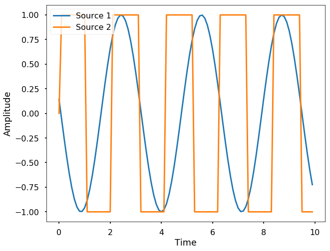
Let's generate two signals and see if we could separate them. We use two different sources, one is a sine wave, and the other one is just a square wave. 
import numpy as np
import matplotlib.pyplot as plt
plt.style.use('seaborn-poster')
%matplotlib inline
t = np.arange(0, 10, 0.1)

s1 = np.sin(2*t + 3)

s2 = np.sign(np.sin(3 * t)) 
Let's plot the two sources:
plt.figure(figsize = (10, 8))
plt.plot(t, s1, label = 'Source 1')
plt.plot(t, s2, label = 'Source 2')
plt.legend(loc = 2)
plt.xlabel('Time')
plt.ylabel('Amplitude')
Text(0,0.5,'Amplitude')
png
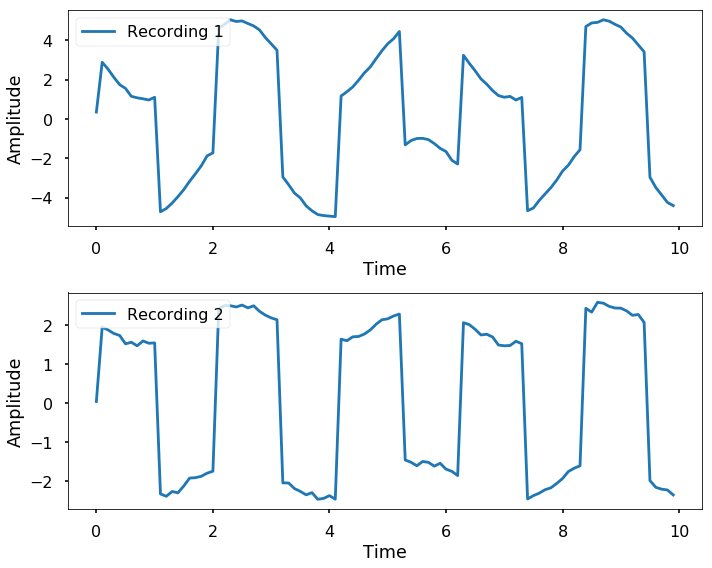
Now let's assume that we have two recorders that recorded the mixture of the two sources, but they emphasize the two sources differently (plus, we add in some white noise as well). 
r1 = 2*s1 + 3*s2 + 0.05* np.random.normal(size=len(t))
r2 = 0.5*s1 + 2*s2 + 0.05 * np.random.normal(size=len(t))
plt.figure(figsize = (10, 8))
plt.subplot(211)
plt.plot(t, r1, label = 'Recording 1')
plt.legend(loc = 2)
plt.xlabel('Time')
plt.ylabel('Amplitude')
plt.subplot(212)
plt.plot(t, r2, label = 'Recording 2')
plt.legend(loc = 2)
plt.xlabel('Time')
plt.ylabel('Amplitude')
plt.tight_layout()
png
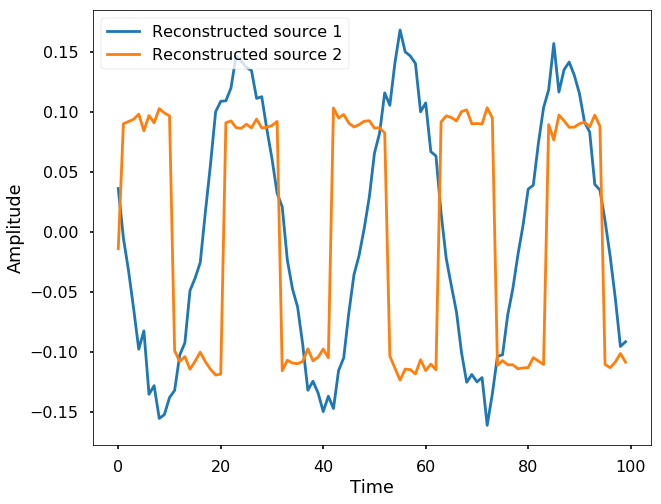
Now let's try to use ICA to separate the two signals. 
from sklearn.decomposition import FastICA
S = np.c_[r1, r2]
S /= S.std(axis=0) 
# Compute ICA
ica = FastICA(n_components = 2, random_state=2)
signal_ica = ica.fit_transform(S)  # Reconstruct signals
A_ = ica.mixing_  # Get estimated mixing matrix
print(A_)
[[4.41784919 8.97120998]
 [1.98294353 9.80142515]]
plt.figure(figsize = (10, 8))
l = plt.plot(signal_ica)
plt.legend(iter(l), ('Reconstructed source 1', 'Reconstructed source 2'), loc = 2)
plt.xlabel('Time')
plt.ylabel('Amplitude')
Text(0,0.5,'Amplitude')
png