In last week's blog, we talked about the basics of Artificial Neural Network (ANN), and gave an intuitive summary and example. Hope you already get a sense of how ANN works. This week, we will continue to explore more of the ANN, and implement a simple version of it so that you will have a better understanding. You can find all the code and the blog material on Qingkai's Github.
After reading this blog, you will understand some key concepts: Inputs, Weights, Outputs, Targets, Activation Function, Error, Bias term, Learning rate.
Let's start with the simple type of Artificial Neural Network - Perceptron, which developed back to the late 1950s; its first implementation, in custom hardware, was one of the first artificial neural networks to be produced. You can also treat it as a two layer neural network without the hidden layers. Even though it has limitations, it contains most of the parts we want to cover for the ANN.
Let's see this example with 4 data sample, this is the input of the data. Each of the samples have 3 features. The target of the data is simply 0 or 1 for two different classes, i.e. class 0, and class 1. We want to build and train a simple Perceptron model that can output the correct target by feeding into the 3 features from the data samples. See the following table. This example is modified from this great post.
| Feature1 | Feature2 | Feature3 | Target |
|---|---|---|---|
| 0 | 0 | 1 | 0 |
| 1 | 1 | 1 | 1 |
| 1 | 0 | 1 | 1 |
| 0 | 1 | 1 | 0 |
Let's have a look of the structure of our model.
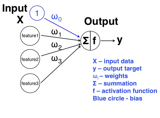
We can see from the figure that we have two layers in this model: the input layer and the output layer. For the input layer, it has 3 features that connect to the output layer via 3 weights. Also we added one more node with 1 as input, and the weight associated with it is the $\omega_0$, we will talk more of this term next. The steps we will take to train this model is: 1. Initialize the weights to small random numbers with both positive or negative values. 2. For many iterations:
Calculate the output value based on all data samples. Update the weights based on the error.
Calculate the output value based on all data samples. Update the weights based on the error.
Before we look at the code how to implement this, we need go through some concepts:
Bias term
Now let's look at the extra 1 we added to the input layer. It is connected to the output layer by weight $\omega_0$. Why we add 1 to the input? Think about the case if all our features are 0, and no matter what weights we have, we will always have 0 to the output layer. Therefore, adding this 1 extra node can avoid this problem. It is usually called bias term.
Activation function
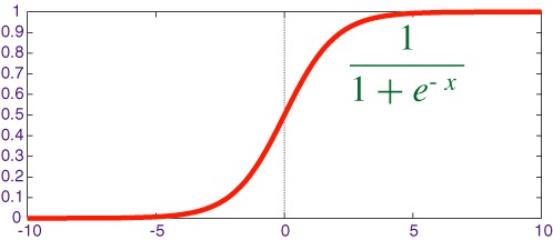
The output layer only has one node, that sum all the passed input and determine whether the output should fire or not (this is ANN terminology related with the brain, when we have enough signal at the neurons, they will fire a signal, the threshold can be different). Usually we use 1 indicate fire and 0 indicate not fire. In this case, we can see the sum of all the input via the weights are: z = $1\omega_0 + feature1\omega1 + feature2*\omega2 + feature3*\omega_3$. But what we want as the output is either 0 or 1 to represent two classes, or a number between 0 and 1, so that we can use it as a probability. Since this number z can be anything, how can we scale it to a value within 0 to 1, as a probability, or simply 0 and 1? Here, the activation function comes to help. The purpose of using the activation function is to achieve this goal. Therefore, we can choose many different activation function, but the most commonly used activation function is the sigmoid (also called logistic) function, which is shown below, to scale the value z to a number between 0 and 1 to represent probability. The advantage of using this function lies in its ability to get the derivative. Since the derivative will be used to update the weights during learning, this property from the sigmoid function is very desirable. The horizontal axis is the z value from the above, it can be any value from negative to positive. The vertical axis is the scaled value from 0 to 1 that we can use as our output. We can see that, if the z value we get is a large positive number, say 10, or a very small negative number, i.e. -10, the scaled value will be either 1 or 0. We can say at these cases, the network is very confident that the class is belong to certain class. But if we have z relatively close to 0, for example, -1 to 1, then the scaled value will be around 0.2 to 0.7, which also indicates the network is not so confident about the result.
Therefore, by input the features to the network, and we can get the perceptron network to classify an object into two different class. But what if the result is wrong by input the features? This is totally possible, since we initialize the weights as random small numbers. To solve this problem, we need the perceptron to have the ability to learn from the data.
How to learn from error
Learning will be achieved by first estimate how much error we make by using current weights, and then find some way to update the weights that we can reduce the error in the next time. I won't say too much here, but we will see more details with the explanation of the following code.
Learning rate
Usually, we also need a learning rate to control how fast the network learns. We will see later in the code that the learning rate decide how much to change the weight by. We could miss it out, which would be the same as setting it to 1. But if we do that, the weights change a lot whenever there is a wrong answer, which tends to make the network unstable, so that it never settles down. The cost of having a small learning rate is that the weights need to see the inputs more often before they change significantly, so that the network takes longer to learn. However, it will be more stable and resistant to noise (errors) and inaccuracies in the data.
Let's look at the code to do the above things to learn from data, and explain them line by line below:
1.  import numpy as np
2.
3.  # The activation function, we will use the sigmoid
4.  def sigmoid(x,deriv=False):
5.      if(deriv==True):
6.          return x*(1-x)
7.      return 1/(1+np.exp(-x))
8.
9.  # define learning rate
10. learning_rate = 0.4
11.
12. # input dataset, note we add bias 1 to the input data
13. X = np.array([[0,0,1],[1,1,1],[1,0,1],[0,1,1]])
14. X = np.concatenate((np.ones((len(X), 1)), X), axis = 1)
15.
16. # output dataset
17. y = np.array([[0,1,1,0]]).T
18.
19. # seed random numbers to make calculation
20. # deterministic (just a good practice)
21. np.random.seed(1)
22.
23. # initialize weights randomly with mean 0
24. weights_0 = 2*np.random.random((4,1)) - 1
25.
26. # train the network with 50000 iterations
27. for iter in xrange(50000):
28.
29.     # forward propagation
30.     layer_0 = X
31.     layer_1_output = sigmoid(np.dot(layer_0,weights_0))
32.
33.     # how much difference? This will be the error of
34.     # our estimation and the true value
35.     layer1_error = y - layer_1_output
36.
37.     # multiply how much we missed by the
38.     # slope of the sigmoid at the values at output layer
39.     # we also multiply the input to take care of the negative case
40.     layer1_delta = learning_rate * layer1_error * sigmoid(layer_1_output,True)
41.     layer1_delta = np.dot(layer_0.T,layer1_delta)
42.
43.     # update weights by simply adding the delta
44.     weights_0 += layer1_delta
45.
46. print "Output After Training:"
47. print layer_1_output
Output After Training:
[[ 0.00596263]
[ 0.99466926]
[ 0.99523979]
[ 0.00532484]]Explain line by line
Line 1: This line imports the numpy module, which is a linear algebra library.
Line 4: This block defines the activation function, which is a function to convert any number to a probability between 0 and 1 as we discussed above.
Line 10: Here we define our learning rate, this will control how fast the network learns from the data. Usually this learning rate will be a number within 0 - 1, with 0 means the network will not learn at all, and 1 means the network will learn a full speed.
Line 13: This initializes the input dataset as numpy matrix. Each row is a single data sample, and each column corresponds to one features (one of the input nodes). And we also add the bias term 1 in line 14. You can see that we now have 4 input nodes and 4 training examples.
Line 17: This initializes our output dataset.
.Tis the transpose function, which to convert our output data to a column vector. You can see that we have 4 rows and 1 column, corresponds to 4 data samples and 1 output node.
Line 21: Before we generate the random weights, we use a seed to make sure that every time we have the same set of random number generated. This is very useful when we test the algorithm, and compare the results with others. This means that your results and my results should be the same. But in reality when you use the algorithm, you don't need to seed it.
Line 24: This initializes our weights to connect the input layer to the output layer. Since we have 4 input nodes (including the bias term), we initialize the random weights as dimension (4,1). Also note that the random numbers we initialized are within -1 to 1, with a mean of 0. There is quite a bit of theory that goes into weight initialization. For now, just take it as a best practice that it's a good idea to have a mean of zero in weight initialization.
Line 27: We begin the training and make the Perceptron to learn in 50000 iterations. In each of the iteration, the algorithm will learn from the error it made.
Line 30: We just explicitly assign out input data to layer0 (since we have 2 layers, we will call it layer0, and layer_1). We're going to process all the data at the same time in this implementation, this is called 'batch processing'. There's another type of learning called 'online learning', which essentially change the weights whenever there's new data sample available, but we won't talk it here.
Line 31: This is the forward propagation. It has two steps, first, the input data from the input layer and propagate to the output layer via the weights, and second, the activation function convert it into a number between 0 and 1. The first step is achieved by the np.dot function, np.dot(layer0,weights0) = $1\omega_0 + feature1\omega1 + feature2*\omega2 + feature3*\omega_3$, we can call the derived number is z. The second step is passing this number z to the sigmoid function to get a number between 0 to 1.
Line 35: This is the error we made using the current weight, it is simply the true answer (y) minus our estimation (layer1output). The error of each of the data sample we input into the network is stored here as a 4 by 1 matrix.
Line 40: This is the most important part - learning. This is the line that makes our algorithm learn from the data. It calculates how much we will change each of the weights in the current iteration. It has 3 parts that multiplied together, (1) the learning rate, (2) the error we just got, and (3) the derivative of the sigmoid function at the output value.
The first term is the learning rate, which controls how fast we will learn, it is just a constant in this case, say, we can choose it as 0.4. The larger the values is, the faster the network will learn, but may make the learning unstable and cause the results oscillating that never get the correct results.
The second term is the error we made. Let's think this error a little more: we have two class, class 0 and class 1. Therefore, we can have two type of error, true class is 0, but our estimation is larger than 0, the other case is true class is 1, but our estimation is less than 1. The error will be a negative number for the first case, but a positive number for the second. If we assume all the input node is positive, and we get an error as negative number, then we want to reduce the weight to make next estimation smaller. Same thing for the other case, if we have the error as a positive number, then we will want to increase the weights, so that in the next iteration, our estimation will be larger. This is the purpose we include the error term here to determine how we change the weights. But wait, what if the input nodes contain negative input? This will switch the values over, and reverse the direction we want to change the weights. How can we avoid this case? Well, it is quite simple, we can just multiply the input into this function, the negative error with negative input multiply will be a positive number, which satisfy our need. This is where line 42 comes in, we separate these two lines for more clear explanation.
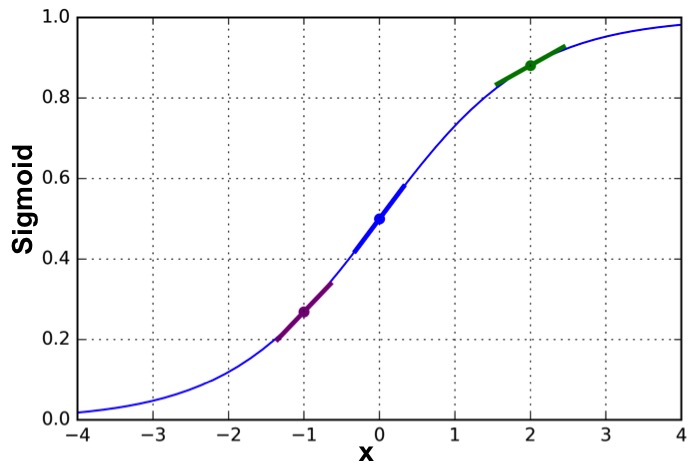
The final term is the derivative of the sigmoid function evaluated at the output value. We can see a simple plot of the sigmoid function and it's derivatives at different places. The derivative at x is the slope of the sigmoid curve at value x. We can clearly see the slope is different at various value x, ranging from 0 (when x value is approaching to two end, i.e. either really large or really small, you can also see the slope is very flat) to 1 (when x value is close to the 0, the slope is very steep). This means we will multiply another value that is between 0 to 1 to the error we made that already scaled with the learning rate. If we look carefully with the figure, the slope of the green and purple dots are flat than the blue dot, which means they will have a smaller value. The green and purple dots represent more confidence of the result to be one class, for example, the green dot the sigmoid value is about 0.9, which is much close to the class 1. But the blue dot has a sigmoid value 0.5, which we have no idea whether it should belong to class 1 or class 0. Therefore, this slope is large when we have no confidence of determine the class of result, and small when we have more confidence of the class of the results. Now, this makes sense, if the current weights already made a very good estimate of the class (for the green dot), we will want to update the weights really small or even not update it. But if the current estimation is not clear, for example, the blue case, we will want to change the weights relatively large to make it clearer. Therefore, combining the 3 terms, we can get a delta value for each of the weight we want to change in the direction to reduce the error.
Line 41: As we talked about the negative input case (see line 39 second term explanation), where we need multiply the input to keep the sign correctly (to keep the direction we want to change the weights correctly!).
Line 44: This is the last line, it aims to update the current weights by simply adding the delta we just determined to the current weights.
Line 47: This line just print out the final results we get after the network learned 50000 iterations, and we can see we get a pretty decent results.
This concludes this blog by showing you all the important part of the ANN (perceptron) algorithm. But the perceptron has its own limation, which actually caused the ANN winter we talked about in the 1970s until researchers found the way to solve it - the multilayer perceptron algorithm, which we will talk in the next blog.
References and Acknowledgments
A Neural Network in 11 lines of Python (I thank the author, since my blog is modified from his blog).
Machine learning - An Algorithmic Perspective
Single-Layer Neural Networks and Gradient Descent
Machine learning - An Algorithmic Perspective
Single-Layer Neural Networks and Gradient Descent
Good post. Check our Digital Weighing Scale
ReplyDelete
ReplyDeleteJust found your post by searching on the Google, I am Impressed and Learned Lot of new thing from your post.
Mehandi Design
Five weeks ago my boyfriend broke up with me. It all started when i went to summer camp i was trying to contact him but it was not going through. So when I came back from camp I saw him with a young lady kissing in his bed room, I was frustrated and it gave me a sleepless night. I thought he will come back to apologies but he didn't come for almost three week i was really hurt but i thank Dr.Azuka for all he did i met Dr.Azuka during my search at the internet i decided to contact him on his email dr.azukasolutionhome@gmail.com he brought my boyfriend back to me just within 48 hours i am really happy. What’s app contact : +44 7520 636249
ReplyDeletehttp://emc-mee.com/transfer-furniture-dammam.html شركة نقل عفش بالدمام
ReplyDeletehttp://emc-mee.com/transfer-furniture-taif.html شركة نقل عفش بالطائف
http://emc-mee.com/transfer-furniture-mecca.html شركة نقل عفش بمكة
http://emc-mee.com/transfer-furniture-yanbu.html شركة نقل عفش بينبع
aedsrg
ReplyDelete