Friday, December 29, 2017

Use K-D Tree to query points - Part 2 (Use geo-coordinates and real distances)

In the previous post, we talked about using KD-tree to find the closest points from a reference point in a group. But we notice that it is using the Euclidean distance. In reality, we use the points on the earth, and want to use the real distance between two points on the earth (at least for me, this is usually the case). Therefore, we need to use the KD-tree with the real distances we usually used in life. In this post, I will tell you how to do it. You can find all the code on Qingkai’s Github.
from scipy import spatial
import numpy as np
import matplotlib.pyplot as plt
from mpl_toolkits.basemap import Basemap
%matplotlib inline

plt.style.use('seaborn-poster')
Let’s first generate a grid of data points in Bay Area with latitude/longitude step 0.1 degree. We can choose the reference point at the center of the map. See the following figure:
# define map ranges
llat = 37.0
ulat = 38.5
llon = -123
ulon = -121.5

# generate grid points
lats = np.arange(llat, ulat, 0.1)
lons = np.arange(llon, ulon, 0.1)
lons, lats = np.meshgrid(lons, lats)

# flatten the locations
lons_1d = lons.flatten()
lats_1d = lats.flatten()

# reference point as the center of the map
lat_0 = (llat + ulat) / 2.
lon_0 = (llon + ulon) / 2.
plt.figure(figsize=(10,10))
m = Basemap(projection='merc', lon_0=-125.36929, lat_0=38.3215, 
        llcrnrlon=llon,llcrnrlat=llat- 0.01,urcrnrlon=ulon,urcrnrlat=ulat + 0.01,resolution='h')
m.drawcoastlines()
m.drawmapboundary()

m.drawparallels(np.arange(llat, ulat + 0.01, (ulat - llat)/2.), labels=[1,0,0,0], linewidth=0.1, fmt='%.1f')
m.drawmeridians(np.arange(llon, ulon + 0.01, (ulon - llon)/2.), labels=[0,0,0,1], linewidth=0.1, fmt='%.1f') 

x_0, y_0 = m(lons_1d, lats_1d)
m.plot(x_0, y_0, 'bo', markersize=10) 

x_0, y_0 = m(lon_0, lat_0)
m.plot(x_0, y_0, 'r*', markersize=30) 

m.fillcontinents()
m.drawmapscale(llon + 0.2, llat + 0.1, lon_0, lat_0, 30, 'fancy')

plt.show()
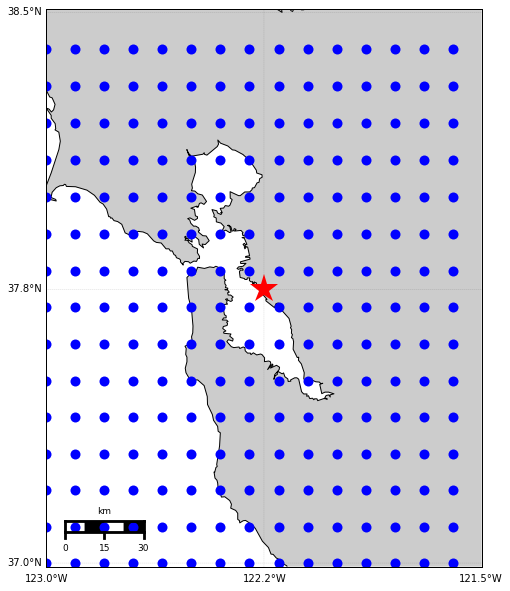
png

Find the points within 30 km from the reference point

Now, let’s find the points within 30 km from the reference points using KD-tree. I got the idea from this discussion at stackoverflow. The basic idea is to convert the latitude and longitude of the points to 3D cartesian coordinates and do the KD-tree query in this cartesian coordinates. We first define the functions to convert the points between the geo-coordinates and the cartesian coordinates.
from math import *

def to_Cartesian(lat, lng):
    '''
    function to convert latitude and longitude to 3D cartesian coordinates
    '''
    R = 6371 # radius of the Earth in kilometers

    x = R * cos(lat) * cos(lng)
    y = R * cos(lat) * sin(lng)
    z = R * sin(lat)
    return x, y, z

def deg2rad(degree):
    '''
    function to convert degree to radian
    '''
    rad = degree * 2*np.pi / 360
    return(rad)

def rad2deg(rad):
    '''
    function to convert radian to degree
    '''
    degree = rad/2/np.pi * 360
    return(degree)

def distToKM(x):
    '''
    function to convert cartesian distance to real distance in km
    '''
    R = 6371 # earth radius
    gamma = 2*np.arcsin(deg2rad(x/(2*R))) # compute the angle of the isosceles triangle
    dist = 2*R*sin(gamma/2) # compute the side of the triangle
    return(dist)

def kmToDIST(x):
    '''
    function to convert real distance in km to cartesian distance 
    '''
    R = 6371 # earth radius
    gamma = 2*np.arcsin(x/2./R) 
    
    dist = 2*R*rad2deg(sin(gamma / 2.))
    return(dist)
# convert the grid points and reference points to cartesian coordinates
x, y, z = zip(*map(to_Cartesian, lats_1d, lons_1d))
x_ref, y_ref, z_ref = to_Cartesian(lat_0, lon_0)
# convert the 30 km to cartesian coordinates distance
dist = kmToDIST(30)

# create the KD-tree using the 3D cartesian coordinates
coordinates = list(zip(x, y, z))
tree = spatial.cKDTree(coordinates)

# get all the points within 30 km from the reference point
ix = tree.query_ball_point((x_ref, y_ref, z_ref), dist)

# plot them on the map
plt.figure(figsize=(10,10))
m = Basemap(projection='merc', lon_0=-125.36929, lat_0=38.3215, 
        llcrnrlon=llon,llcrnrlat=llat- 0.01,urcrnrlon=ulon,urcrnrlat=ulat + 0.01,resolution='h')
m.drawcoastlines()
m.drawmapboundary()

m.drawparallels(np.arange(llat, ulat + 0.01, (ulat - llat)/2.), labels=[1,0,0,0], linewidth=0.1, fmt='%.1f')
m.drawmeridians(np.arange(llon, ulon + 0.01, (ulon - llon)/2.), labels=[0,0,0,1], linewidth=0.1, fmt='%.1f') 

x_0, y_0 = m(lons_1d, lats_1d)
m.plot(x_0, y_0, 'bo', markersize=10, label = 'Grid point') 

x_0, y_0 = m(lon_0, lat_0)
m.plot(x_0, y_0, 'r*', markersize=30, label = 'Ref. point') 

x_0, y_0 = m(lons_1d[ix], lats_1d[ix])
m.plot(x_0, y_0, 'ro', markersize=10, label = 'Point within 30 km') 

m.fillcontinents()
m.drawmapscale(llon + 0.2, llat + 0.1, lon_0, lat_0, 30, 'fancy')

plt.legend(numpoints = 1)

plt.show()
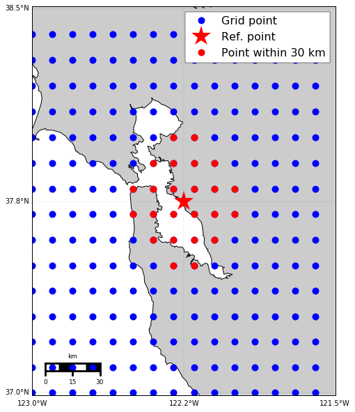
png

Find the distances for the closest 10 points

We can also find the distances from the closest 10 points. This will be very simple by using the query function.
# get the cartesian distances from the 10 closest points
dist, ix = tree.query((x_ref, y_ref, z_ref), 10)

# print out the real distances in km
print(map(distToKM, dist))
[7.849314101994533, 7.849314102001198, 7.859304141667372, 7.859304141674064, 17.516008198378657, 17.516008198387585, 17.547633149227252, 17.547633149230194, 17.55621138531865, 17.556211385327607]
Wednesday, December 27, 2017

Use K-D Tree to query points - Part 1

We have a group of 2D points, for example, group A, contains 50 data points. We have another point B (or another group of points), that we want to find n points in A that are closest to the point in B. How do we do that? The simplest thinking is that, we can calculate the distances of all the points from A to B and decide which are the closest n points.
But wait a minute, this sounds we need to do a lot of work. For example, if we want to find the 1 closest countries from US, do we need to calculate all the countries in the southern hemisphere? Are there any good ways that we don’t need to calculate all the distances? Yes, there is a way! This is what I want to show this week - K-D tree. I won’t go into details of this algorithm, if you are interested, you can find the intuition here.
I will use a python example to show how easy to use K-D tree to do the job. You can find the code on Qingkai's Github. But you will notice that the distance here is just Euclidean distance, what if we want to use the distance on earth? We will show that in part 2 in the next post. 
from scipy import spatial
import numpy as np
import matplotlib.pyplot as plt

%matplotlib inline

plt.style.use('seaborn-poster')
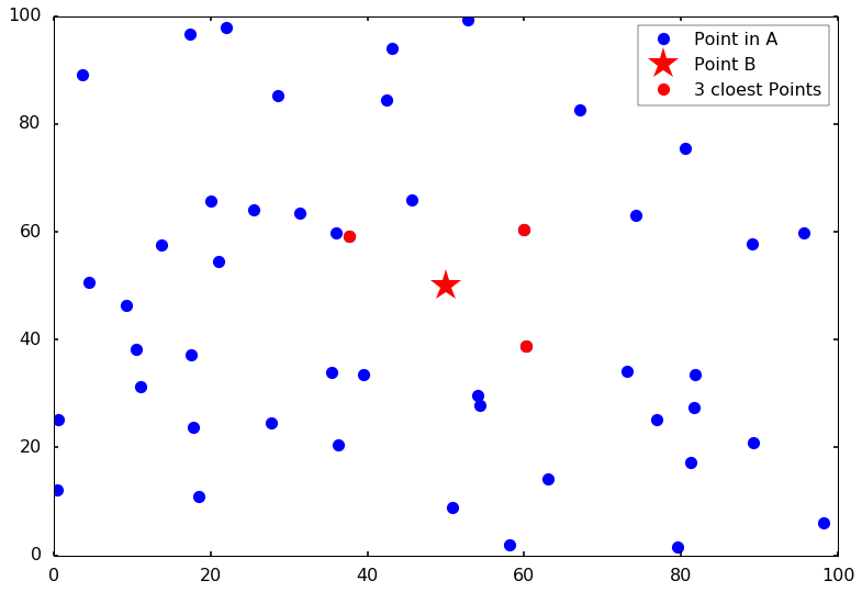
Let’s first generate 50 x and y points in group A and for simplicity, generate one point in group B. We will calculate the 3 closest data points from A to B.
np.random.seed(100)
A = np.random.random((50,2))*100

B = [50, 50]
We first build the K-D tree using the function in scipy. And query the 3 closest points to B. Note that, the distance here is the Euclid distance.
# we use cKDTree instead of KDTree, since it is a C version, will be faster. 
kdtree = spatial.cKDTree(A)

# it returns the distance and the index of the points, 3 means we want the top 3 cloest points
dist, ix = kdtree.query(B, 3)
plt.plot(A[:, 0], A[:, 1], 'o', label = 'Point in A')
plt.plot(B[0], B[1], 'r*', markersize = 30, label = 'Point B')
plt.plot(A[:, 0][ix], A[:, 1][ix], 'ro', label = '3 cloest Points')
plt.legend(numpoints = 1)
plt.show()
png

Find all points within certain distance

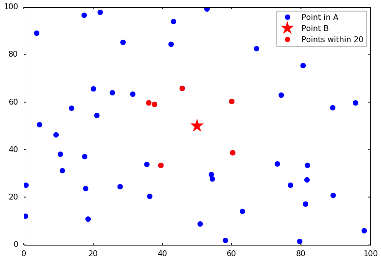
We can also ask the question: ‘what are the points within distance 20 from B’. Here is how we do it:
# let's find all the points within distance 20 from point B
ix_list = kdtree.query_ball_point(B, 20)
plt.plot(A[:, 0], A[:, 1], 'o', label = 'Point in A')
plt.plot(B[0], B[1], 'r*', markersize = 30, label = 'Point B')
plt.plot(A[:, 0][ix_list], A[:, 1][ix_list], 'ro', label = 'Points within 20')
plt.legend(numpoints = 1)
plt.show()
png

Find all pairs within certain distance

If you have another group of points, you can find all the points in one group within distance 10 from another group. I will just use group A to itself, basically, we will find all the pairs of data points that has distance within 10. You can see that for each point, itself is included in the returned index, because the distance is 0.
kdtree.query_ball_tree(kdtree, 10)
[[0, 45],
 [1, 10],
 [2],
 [3],
 [4, 22],
 [5, 8, 9],
 [6],
 [7, 36],
 [5, 8, 23],
 [5, 9, 11, 23],
 [1, 10],
 [9, 11, 23, 38],
 [12, 16, 46],
 [13],
 [14],
 [15],
 [12, 16, 39, 46],
 [17],
 [18],
 [19, 37],
 [20],
 [21, 40],
 [4, 22],
 [8, 9, 11, 23, 38],
 [24],
 [25, 32],
 [26, 30, 44],
 [27, 42],
 [28, 35],
 [29, 39],
 [26, 30, 44],
 [31],
 [25, 32],
 [33],
 [34, 35],
 [28, 34, 35],
 [7, 36],
 [19, 37],
 [11, 23, 38],
 [16, 29, 39],
 [21, 40],
 [41],
 [27, 42],
 [43],
 [26, 30, 44, 48],
 [0, 45],
 [12, 16, 46],
 [47],
 [44, 48, 49],
 [48, 49]]

Sunday, December 24, 2017

Create discrete colormap

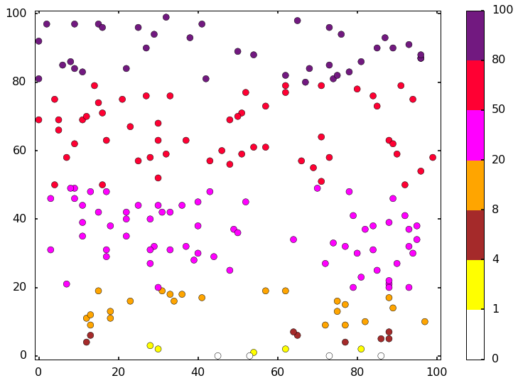
Many times, we need different color scales to emphasize different parts. But sometimes, we want to specify some color maps by ourselves, there are ways to do this. Also, sometimes, we want to specify some colors bins, and if my value falls into the bin, I use one specific color. For example, I want the following color schema:
  • 0 <= v < 1, white
  • 1 <= v < 4, yellow
  • 4 <= v < 8, brown
  • 8 <= v < 20, orange
  • 20 <= v < 50, magenta
  • 50 <= v < 80, #FF0033 (sort of red)
  • 80 <= v < 100, #721980 (purple)
In the following, I will give an example, you can find the notebook on Qingkai's Github
import numpy as np
import matplotlib.pyplot as plt
import matplotlib.colors as colors
%matplotlib inline
plt.style.use('seaborn-poster')
# generate x and y value between [0, 100)
np.random.seed(10)
x = np.random.randint(low = 0, high=100, size=200)
y = np.random.randint(low = 0, high=100, size=200)
# set colors
colorsList = ['white', 'yellow', 'brown', 'orange', 'magenta', '#FF0033', '#721980']
CustomCmap = colors.ListedColormap(colorsList)
bounds = np.array([0, 1, 4, 8, 20, 50, 80, 100])
norm = colors.BoundaryNorm(boundaries=bounds, ncolors=7)
plt.scatter(x,y,c=y, s = 80, cmap=CustomCmap, norm = norm)
plt.colorbar()
plt.ylim(-1,101)
plt.xlim(-1,101)
plt.show()
png

Thursday, December 21, 2017

What is ablation study in machine learning

We often come across 'ablation study' in machine learning papers, for example, in this paper with the original R-CNN, it has a section of ablation studies. But what does this means?

Well, we know that when we build a model, we usually have different components of the model. If we remove some component of the model, what's the effect on the model? This is a very coarse definition of ablation study - we want to see the contributions of some proposed components in the model by comparing the model including this component with that without this component.

In the above paper, in order to see the effect of fine-tuning of the CNN, the authors analyzed the performance of the model with the fine-tuning and the performance of it without the fine-tuning. This way, we can easily see the effect of the fine-tuning.

The following I copied from the answer of Jonathan Uesato on Quora, it explains very well:

An ablation study typically refers to removing some “feature” of the model or algorithm and seeing how that affects performance.
Examples:
  • An LSTM has 4 gates: feature, input, output, forget. We might ask: are all 4 necessary? What if I remove one? Indeed, lots of experimentation has gone into LSTM variants, the GRU being a notable example (which is simpler).
  • If certain tricks are used to get an algorithm to work, it’s useful to know whether the algorithm is robust to removing these tricks. For example, DeepMind’s original DQN paper reports using (1) only periodically updating the reference network and (2) using a replay buffer rather than updating online. It’s very useful for the research community to know that both these tricks are necessary, in order to build on top of these results.
  • If an algorithm is a modification of a previous work, and has multiple differences, researchers want to know what the key difference is.
  • Simpler is better (inductive prior towards simpler model classes). If you can get the same performance with two models, prefer the simpler one.

Sunday, December 17, 2017

AGU 2017 at New Orleans

I was at AGU 2017 this week, it was held at New Orleans this time (finally not in San Fransisco anymore). It is a great conference overall, and here are some photos I took: